Quantum Experiments - Heisenberg’s Uncertainty Principle

What did Heisenberg really mean by the uncertainty principle?

The most popular form of the uncertainty principle is about position and momentum of a particule, if one is know the other is uncertain; We will examine the same but not the momentum and position but using different basis of measures.

from qiskit import QuantumCircuit, assemble, Aer
from math import pi, sqrt
from qiskit.visualization import plot_bloch_multivector, plot_histogram
sim = Aer.get_backend('aer_simulator')

# Let's do an X-gate on a |0> qubit
qc = QuantumCircuit(1)
qc.x(0)
qc.draw()

   ┌───┐
q: ┤ X ├
   └───┘

# Let's see the result
qc.save_statevector()
state = sim.run(qc).result().get_statevector()
plot_bloch_multivector(state)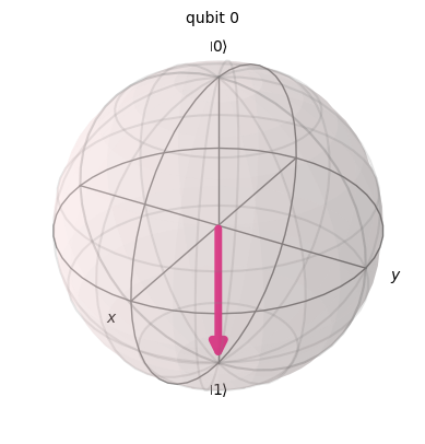

The state hs been changed from 0 to 1, thats what X gate does

qc.y(0) # Do Y-gate on qubit 0
qc.z(0) # Do Z-gate on qubit 0
qc.draw()

   ┌───┐ statevector ┌───┐┌───┐
q: ┤ X ├──────░──────┤ Y ├┤ Z ├
   └───┘      ░      └───┘└───┘

# Create the X-measurement function:
def x_measurement(qc, qubit, cbit):
    """Measure 'qubit' in the X-basis, and store the result in 'cbit'"""
    qc.h(qubit)
    qc.measure(qubit, cbit)
    return qc

initial_state = [1/sqrt(2), -1/sqrt(2)]
# Initialize our qubit and measure it
qc = QuantumCircuit(1,1)
qc.initialize(initial_state, 0)
x_measurement(qc, 0, 0)  # measure qubit 0 to classical bit 0
qc.draw()

     ┌──────────────────────────────┐┌───┐┌─┐
  q: ┤ Initialize(0.70711,-0.70711) ├┤ H ├┤M├
     └──────────────────────────────┘└───┘└╥┘
c: 1/══════════════════════════════════════╩═
                                           0

counts = sim.run(qc).result().get_counts()  # Do the simulation, returning the state vector
plot_histogram(counts)  # Display the output on measurement of state vector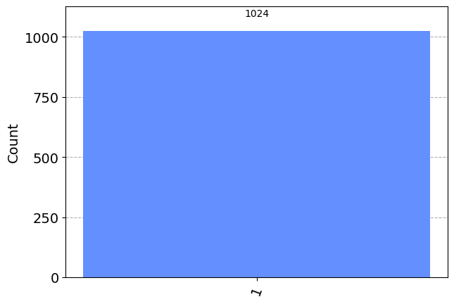

We initialized our qubit in - the state , but we can see that, after the measurement, we have collapsed our qubit to the 1 state . If you run the cell again, you will see the same result, since along the X-basis, the state - is a basis state and measuring it along X will always yield the same result.

Measuring in different bases allows us to see Heisenberg’s famous uncertainty principle in action. Having certainty of measuring a state in the Z-basis removes all certainty of measuring a specific state in the X-basis, and vice versa. A common misconception is that the uncertainty is due to the limits in our equipment, but here we can see the uncertainty is actually part of the nature of the qubit.

Heisenberg’s Uncertainty principle

https://github.com/qiskit-community/qiskit-textbook/blob/main/content/ch-states/old-unique-properties-qubits.ipynb

from qiskit import *
from qiskit.visualization import plot_histogram
%config InlineBackend.figure_format = 'svg' # Makes the images look nice

measure_z = QuantumCircuit(1,1)
measure_z.measure(0,0)

measure_z.draw(output='mpl')

measure_x = QuantumCircuit(1,1)
measure_x.h(0)
measure_x.measure(0,0)

measure_x.draw(output='mpl')

qc_0 = QuantumCircuit(1)

qc_0.draw(output='mpl')

qc = QuantumCircuit.compose(measure_z, qc_0)

qc.draw()

     ┌─┐
  q: ┤M├
     └╥┘
c: 1/═╩═
      0

sim = Aer.get_backend('aer_simulator')
counts = sim.run(qc).result().get_counts()

counts

{'0': 1024}

print('Results for z measurement:')

plot_histogram(counts)

Results for z measurement:

qc = QuantumCircuit.compose(measure_x, qc_0)
sim = Aer.get_backend('aer_simulator')
counts = sim.run(qc).result().get_counts()
qc.draw()

     ┌───┐┌─┐
  q: ┤ H ├┤M├
     └───┘└╥┘
c: 1/══════╩═
           0

print('Results for x measurement:')
plot_histogram(counts)

Results for x measurement:

qc_plus = QuantumCircuit(1)
qc_plus.h(0)

qc_plus.draw(output='mpl')

qc = QuantumCircuit.compose(qc_plus, measure_z)


counts = counts = sim.run(qc).result().get_counts()
qc.draw()

     ┌───┐┌─┐
  q: ┤ H ├┤M├
     └───┘└╥┘
c: 1/══════╩═
           0

print('Results for z measurement:')
plot_histogram(counts)

Results for z measurement:

qc = QuantumCircuit.compose(qc_plus, measure_x)
counts = counts = sim.run(qc).result().get_counts()
qc.draw()

     ┌───┐┌───┐┌─┐
  q: ┤ H ├┤ H ├┤M├
     └───┘└───┘└╥┘
c: 1/═══════════╩═
                0

print('Results for x measurement:')
plot_histogram(counts)

Results for x measurement:

These results hint at an important principle: Qubits have a limited amount of certainty that they can hold. This ensures that, despite the different ways we can extract outputs from a qubit, it can only be used to store a single bit of information. In the case of the blank circuit, this certainty was dedicated entirely to the outcomes of z measurements. For the circuit with a single Hadamard, it was dedicated entirely to x measurements. In this case, it is shared between the two.

Other rotations

qc_y = QuantumCircuit(1)
qc_y.ry( -3.14159/4,0)

qc_y.draw(output='mpl')

qc = QuantumCircuit.compose(qc_y, measure_z)

counts = counts = sim.run(qc).result().get_counts()
qc.draw()

     ┌─────────────┐┌─┐
  q: ┤ Ry(-0.7854) ├┤M├
     └─────────────┘└╥┘
c: 1/════════════════╩═
                     0

print('Results for z measurement:')
plot_histogram(counts)

Results for z measurement:

Here we have a case that we have not seen before. The z measurement is most likely to output 0, but it is not completely certain. A similar effect is seen below for the x measurement: it is most likely, but not certain, to output 1.

qc = QuantumCircuit.compose(qc_y, measure_x)
counts = counts = sim.run(qc).result().get_counts()
qc.draw()

     ┌─────────────┐┌───┐┌─┐
  q: ┤ Ry(-0.7854) ├┤ H ├┤M├
     └─────────────┘└───┘└╥┘
c: 1/═════════════════════╩═
                          0

print('Results for x measurement:')
plot_histogram(counts)

Results for x measurement: